<< BACK

Innovative Tools

Energy Saving

A simple technique with which to achieve the desired average temperatures in greenhouse crop cultivation is implemented in Macqu. A tool is made available to exploit the interaction between photosynthesis and growth at grower’s intuition, as this interaction is not well known for most plants. The method is based on varying the heating set points (i.e. control policy) using past information in order to achieve the desired average for any user-defined period. In determining the control policy no advance weather information is required. The grower can also set safety limits as the ultimate minimum and maximum temperatures allowed. Finally the integration method can coexist with periods of specified set point tracks. In that way the grower is able to implement his fixed policy at certain times of the day while allowing the algorithm freedom to attain the target averages during free periods.

The proposed technique is implemented by combining the tools provided in the MACQU intelligent control system to achieve effective savings in heating. The method combines time-integrated variables and set point generating and tracking techniques in order to store greenhouse heat during favorable periods (sunny days in winter time) and to postpone heating operations during the night by lowering the heating set point.

A static energy balance of a greenhouse can be written in the form:

                                                                  (1)

The first term rS_o represents the net heat input from solar radiation, H is the heat input from heater operation and the third term refers to heat losses. The total heat loss coefficient, U, accounts for all heat losses (conduction, convection, air exchange and re-radiation) and thus is a variable parameter, depending on wind speed and other climatic conditions. T_i  and T_o  are the inner and outer temperatures of the greenhouse respectively.

The course of short, medium and long period inner temperatures has been the subject of substantial research for plant temperature responses. For the long period (crop cycle) policy, static plant production models can be used to pre-compute economical optimum set points for each growth stage. Given the uncertainties of such methods, their accuracy compared with the accumulated unstructured knowledge of expert growers is in question. In this study it is assumed that an external process (optimal off-line programs or grower’s policy) define the long period objectives. The “virtual week” average is introduced requiring definition of the integration period w of the plant (one, two, three or more days) and of the desired temperature integral, T_w. The relation of accumulated average, , for set point control is:

                                        (2)

The left inequality in Eq. 2 is satisfied by use of heating and the right by use of ventilation (constraint satisfaction control). The right equation is used to compute ventilation set point (T.VSP) and the left for heating set point (T.HSP). The later will modulate Ti(t) to assure that the temperature average of the elapsed period w, will be exactly T_wmin , for minimum energy use. This is a post-compensation mechanism. Regardless of which method is used to find an economical optimum T_w, the constraints of Eq. 2 should be examined for validity or corrective actions at appropriate times. When weather information is predicted and forecast w_n period ahead, heating may be scheduled to be more effective, by using an optimization search method which satisfies:

                                                        (3)

where w_p=w-w_n , and minimize accumulated heat gain, Q_w:

                                 (4)

Minimization of Eq. 4, under the constrain of Eq.3, can be used to derive the predicted optimal setpoints T_i(t+j) for 0<j<w_n. Given the fact that weather predictions often fail, application of Eq. 2 is necessary for post-detection compensation. If T_w is allowed to deviate positively to some upper limit T_wmax, to gain free heat when available from solar radiation, the margins for further savings by prediction, compared to post-compensation only, are becoming small. It is worthwhile to conduct a comparative simulated study to assess the importance of forecasted weather for energy saving, under different weather conditions and prediction success probabilities.

Given the linearity of Eq. 2 the week can be segmented into smaller intervals (i.e. days or shorter) so that this expression can be expanded to partial sums as follows:

     (5)

where is the average T_i in the time interval w_j . In the same way Eq. 5 becomes:

             (6)

If U_j is assumed constant, this will lead to a uniform time distribution of applied heat, which is inferior to optimal with regards to efficiency of application. However on the average of longer periods, days or weeks, this assumption will let us draw conclusions on the medium term policy without loss. With this simplification Eq. 6 would give:

              (7)

The result of Eq. 7 simply verifies the fact that the amount of heat input to the greenhouse for one “week” depends on the accumulated inner  degreehours, (in Kh), and the degreehours available outside .

Example of temperature setpoint using the “Temperature Integration” energy saving method.

Installation where the energy saving method is applied

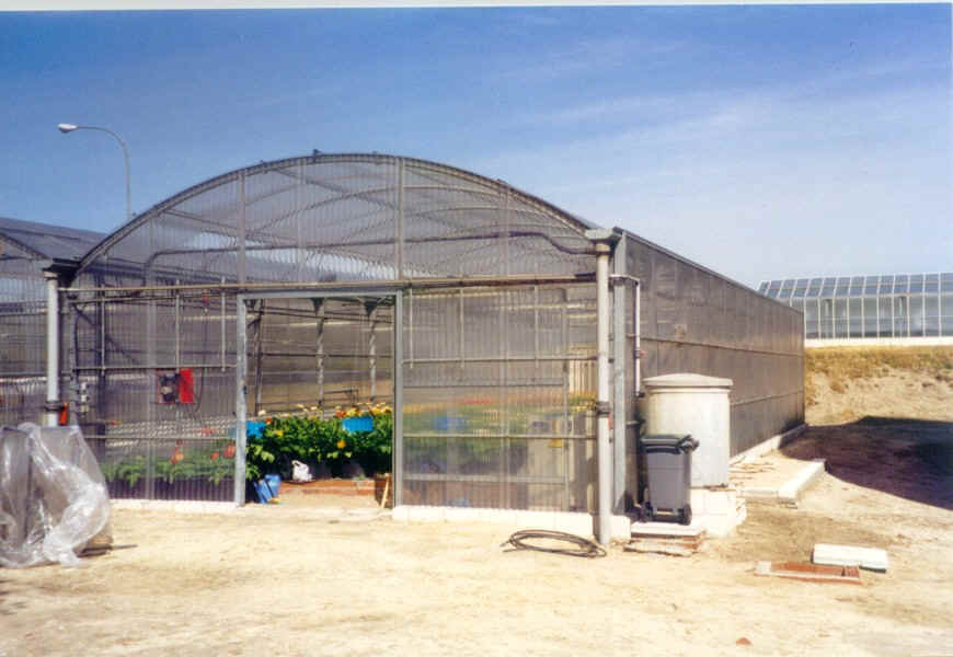Papanikolaoy brothers nurseries Marathon GREECE	Polytechinc University of Madrid Madrid SPAIN

Description of the method with multimedia animations